Chaitanya Belwal's Blog

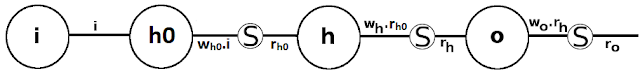
In part-II , we derived the back-propagation formula using a simple neural net architecture using the Sigmoid activation function. In this article, which is a follow on to part-II we expand upon the NN architecture, to add one more hidden layer and derive a generic backpropagation equation that can be applied to deep (multi-layered) neural networks. This article attempts to explain back-propagation in an easier fashion with a simple NN, where each steps has been expanded in great detail and has explanations. After reading this text readers are encouraged to understand the more complex derivations given in Mitchell's book and elsewhere, to fully grasp the concept of back-propagation. You do need a basic understanding of partial derivatives and one of the best explanations are available in videos by Sal Khan at Khan academy . The neural network which has 1 input, 2 hidden and 1 output units(neuron) along with the sigmoid activation function at each hidden and output layer, is gi

In part-II of this article, we derived the weight update equation for the backpropagation operation of a simple Convolutional Neural Network (CNN). The input for the CNN considered in part-II is a grayscale image, hence, the input is in the form of a single 4x4 matrix. CNNs used in practice however, use color images where each of the Red, Green and Blue (RGB) color spectrums serve as input. Hence, a CNN with the inputs color coded with their respective spectrums look like: In this article we expand upon the original CNN where the input is represented by 3, 4x4 matrices each presenting the pixel intensities for the RGB color spectrum. Hence is we represent each of the pixels with the CNN given is represented by: In this CNN, there are 3, 4x4 input matrices, one 2x2 filter matrix (also known as kernel), a single convolution layer with 1 unit, a single ReLu layer, a single pooling layer (which applies the MaxPool function) and a single fully connected (FC) layer. The elements

Ever since  Guido van Rossum introduced Python in 1991, it has  arguably become the favorite programming language for both programmers and non-professional programmers. While Python is used extensively in scientific and data computing, with it's easy extensibility and availability of several packages, it is also a handy tool for doing operating system scripting jobs which are usually done by sh/bash scripts in Unix flavor operating systems and by batch (*.bat) scripts in Windows. In this article, we take a look a simple Python script which replaces a Window batch script and is scheduled to run weekly through the Windows tasks scheduler. The original batch script takes weekly backup of a folder into an external drive. Only one copy of the backup folder is required hence the existing backup folder is deleted before the copy (this to ensure there is space for copying the new folder). The backup folder should also be inside folder(s) that represent the date the copy was made. T

In part-I of this article, we derived the weight update equation for a backpropagation operation of a simple Convolutional Neural Network (CNN). The CNN considered in part-I did not use a rectified linear unit (ReLu) layer, and in this article we expand upon the CNN to include a ReLu layer and see how it impacts the backpropagation. The CNN we use in this article is given below: In this simple CNN, there is one 4x4 input matrix, one 2x2 filter matrix (also known as kernel), a single convolution layer with 1 unit, a single ReLu layer, a single pooling layer (which applied the MaxPool function) and a single fully connected (FC) layer. The elements of the filter matrix are equivalent to the unit weights in a standard NN and will be updated during the backpropagation phase. Assuming a stride of 2 with no padding, the size of the convolution layer is determined by the following equation: $$ N={(W - F + 2.P)\over S} + 1 $$ Here, N : is the dimension (rows and columns) of

In another article, we explained the basic mechanism of how a Convolutional Neural Network (CNN) works. In this article we explain the mechanics backpropagation w.r.t to a CNN and derive it value. We use the same simple CNN as used int he previous article, except to make it more simple we remove the ReLu layer. In part-II of this article we derive the backpropagation in the same CNN with the addition of a ReLu layer. The CNN we use is given below: In this simple CNN, there is one 4x4 input matrix, one 2x2 filter matrix (also known as kernel), a single convolution layer with 1 unit, a single pooling layer (which applied the MaxPool function) and a single fully connected (FC) layer. The elements of the filter matrix are equivalent to the unit weights in a standard NN and will be updated during the backpropagation phase. Assuming a stride of 2 with no padding, the size of the convolution layer is determined by the following equation: $$ N={(W - F + 2.P)\over S} + 1 $$ He